Natural spline LME model in lme4
Natural spline LME model in lme4
Ahmed Elhakeem 2026-04-21
- Clear the Work Environment
- Install Packages (if needed)
- Load Packages
- Load BMI Data Set
- 1 – Natural Spline LME: Females
- 2 – Natural Spline LME: Males
- 3 – Natural Spline LME: Males and Females
Clear the Work Environment
rm(list = ls())
Install Packages (if needed)
install.packages(c("broom.mixed", "tidyverse", "lme4", "ggeffects",
                   "splines", "marginaleffects", "emmeans", "mgcv"))
Load Packages
library(broom.mixed)
library(marginaleffects)
library(tidyverse)
library(ggeffects)
library(emmeans)
library(splines)
library(lme4)
Load BMI Data Set
dat <- read.csv(
  "https://raw.githubusercontent.com/aelhak/ARMSC23/main/bmi_long.csv"
) %>%
  mutate(id = as.factor(id), sex = as.factor(sex))
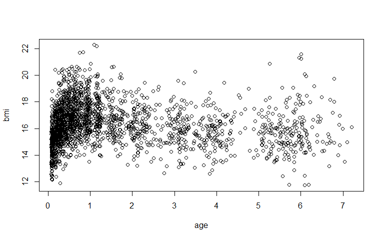
Quick Look at the Data
with(dat, plot(age, bmi))
dat %>% group_by(sex) %>% summarise(N = n_distinct(id))
## # A tibble: 2 × 2
##   sex       N
##   <fct> <int>
## 1 F       100
## 2 M       100
dat %>%
  group_by(id) %>%
  count() %>%
  ungroup() %>%
  summarise(median(n), min(n), max(n))
## # A tibble: 1 × 3
##   `median(n)` `min(n)` `max(n)`
##         <dbl>    <int>    <int>
## 1          11        1       21
Create Sex-Stratified Datasets
dat_m <- dat %>% filter(sex == "M")
dat_f <- dat %>% filter(sex == "F")
1 – Natural Spline LME: Females
Fit natural spline mixed effects models with 3–6 degrees of freedom and select the best model using BIC.
ns_f <- map(3:6, possibly(~ {
  eval(parse(text = paste0(
    "lmer(bmi ~ ns(age, ", .x, ") + (age | id),
    REML = F, data = dat_f)"
  )))
}, otherwise = NA_real_))

(ns_f_best <- ns_f[[which.min(unlist(map(ns_f, BIC)))]])
## Linear mixed model fit by maximum likelihood  ['lmerMod']
## Formula: bmi ~ ns(age, 4) + (age | id)
##    Data: dat_f
##       AIC       BIC    logLik -2*log(L)  df.resid
##  2582.652  2627.192 -1282.326  2564.652      1033
## Random effects:
##  Groups   Name        Std.Dev. Corr
##  id       (Intercept) 1.2190
##           age         0.2742   -0.35
##  Residual             0.6523
## Number of obs: 1042, groups:  id, 100
## Fixed Effects:
## (Intercept)  ns(age, 4)1  ns(age, 4)2  ns(age, 4)3  ns(age, 4)4
##     14.6063       2.5982      -0.3776       3.4593       0.5901
Knot Positions
attr(terms(ns_f_best), "predvars")
## list(bmi, ns(age, knots = c(0.351519158, 0.838830521, 2.24447183625
## ), Boundary.knots = c(0.076364751, 6.916836223), intercept = FALSE))
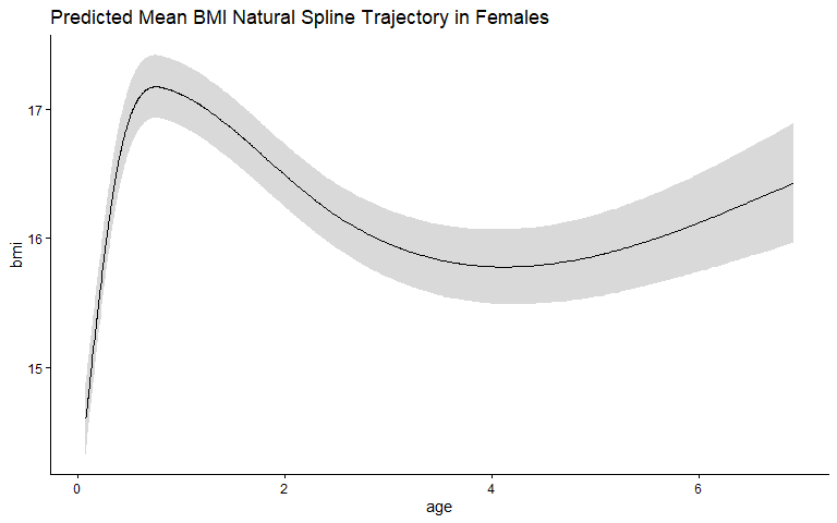
Predicted Mean BMI Trajectory – Females
predict_response(ns_f_best,
                 terms  = c("age [all]"),
                 margin = "marginalmeans") %>%
  plot() +
  ggtitle("Predicted Mean BMI Natural Spline Trajectory in Females") +
  theme_classic()
2 – Natural Spline LME: Males
Fit natural spline mixed effects models with 3–6 degrees of freedom and select the best model using BIC.
ns_m <- map(3:6, possibly(~ {
  eval(parse(text = paste0(
    "lmer(bmi ~ ns(age, ", .x, ") + (age | id),
    REML = F, data = dat_m)"
  )))
}, otherwise = NA_real_))

(ns_m_best <- ns_m[[which.min(unlist(map(ns_m, BIC)))]])
## Linear mixed model fit by maximum likelihood  ['lmerMod']
## Formula: bmi ~ ns(age, 6) + (age | id)
##    Data: dat_m
##       AIC       BIC    logLik -2*log(L)  df.resid
##  2672.910  2727.453 -1325.455  2650.910      1041
## Random effects:
##  Groups   Name        Std.Dev. Corr
##  id       (Intercept) 1.2521
##           age         0.2954   -0.32
##  Residual             0.6689
## Number of obs: 1052, groups:  id, 100
## Fixed Effects:
## (Intercept)  ns(age, 6)1  ns(age, 6)2  ns(age, 6)3  ns(age, 6)4  ns(age, 6)5
##     14.9672       2.1894       2.5570       1.4127      -0.2691       2.4643
## ns(age, 6)6
##     -0.1753
Knot Positions
attr(terms(ns_m_best), "predvars")
## list(bmi, ns(age, knots = c(0.2545100625, 0.468764600333333,
## 0.78427165, 1.49894777866667, 3.50837651933333), Boundary.knots = c(0.07630629,
## 7.208082142), intercept = FALSE))
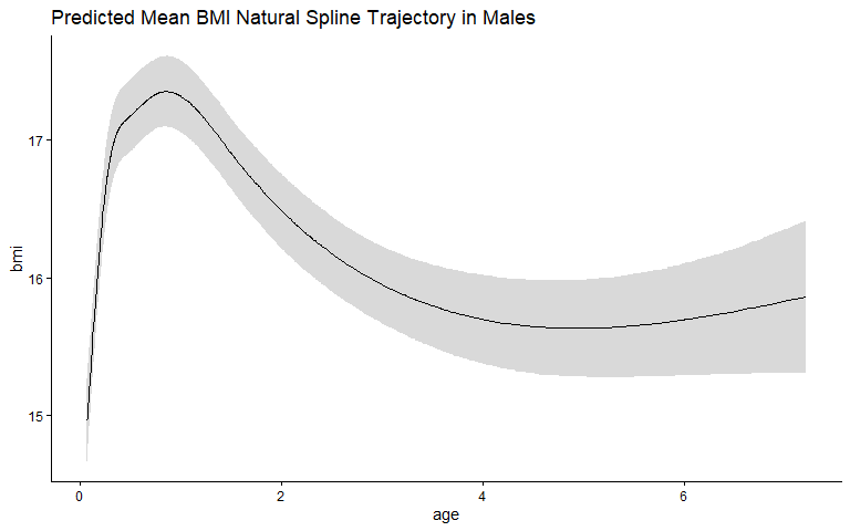
Predicted Mean BMI Trajectory – Males
predict_response(ns_m_best,
                 terms  = c("age [all]"),
                 margin = "marginalmeans") %>%
  plot() +
  ggtitle("Predicted Mean BMI Natural Spline Trajectory in Males") +
  theme_classic()
3 – Natural Spline LME: Males and Females
Fit models with 3–6 df including interactions between age and sex, and select the model with the lowest BIC.
ns_mf <- map(3:6, possibly(~ {
  eval(parse(text = paste0(
    "lmer(bmi ~ ns(age, ", .x, ") * sex + (age | id),
    REML = F, data = dat)"
  )))
}, otherwise = NA_real_))

(ns_mf_best <- ns_mf[[which.min(unlist(map(ns_mf, BIC)))]])
## Linear mixed model fit by maximum likelihood  ['lmerMod']
## Formula: bmi ~ ns(age, 5) * sex + (age | id)
##    Data: dat
##       AIC       BIC    logLik -2*log(L)  df.resid
##  5261.728  5352.078 -2614.864  5229.728      2078
## Random effects:
##  Groups   Name        Std.Dev. Corr
##  id       (Intercept) 1.2348
##           age         0.2846   -0.33
##  Residual             0.6632
## Number of obs: 2094, groups:  id, 200
## Fixed Effects:
##      (Intercept)       ns(age, 5)1       ns(age, 5)2       ns(age, 5)3
##         14.59730           2.81813           2.08979           0.05257
##      ns(age, 5)4       ns(age, 5)5              sexM  ns(age, 5)1:sexM
##          2.98414           1.03194           0.48497          -0.45665
## ns(age, 5)2:sexM  ns(age, 5)3:sexM  ns(age, 5)4:sexM  ns(age, 5)5:sexM
##         -0.32209          -0.66083          -0.65169          -1.22333
Knot Positions
attr(terms(ns_mf_best), "predvars")
## list(bmi, ns(age, knots = c(0.2833373708, 0.5807503106, 1.126253912,
## 3.0883893664), Boundary.knots = c(0.07630629, 7.208082142), intercept = FALSE),
##     sex)
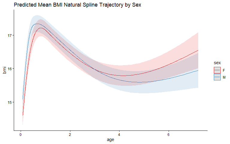
Predicted Mean BMI Trajectory by Sex
predict_response(ns_mf_best,
                 terms  = c("age [all]", "sex [all]"),
                 margin = "marginalmeans") %>%
  plot() +
  ggtitle("Predicted Mean BMI Natural Spline Trajectory by Sex") +
  theme_classic()
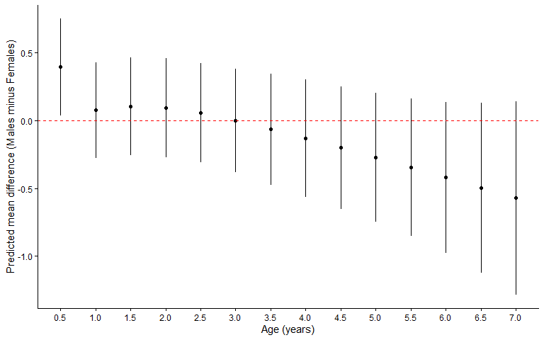
Mean Difference in Predicted BMI (Males minus Females) by Age
pred_diff <- comparisons(
  ns_mf_best,
  variables = "sex",
  newdata   = datagrid(age = seq(0.5, 7, by = 0.5))
) %>% as.data.frame()

ggplot(data = pred_diff,
       aes(x = age, y = estimate, ymin = conf.low, ymax = conf.high)) +
  theme_classic() +
  geom_pointrange(size = 0.25) +
  geom_hline(yintercept = 0, lty = 2, col = "red", linewidth = 0.1) +
  scale_x_continuous(breaks = seq(0.5, 7, by = 0.5)) +
  xlab("Age (years)") +
  ylab("Predicted mean difference (Males minus Females)")