Natural Spline LME Models with lme4 -

Setup
Load and Explore the Data
- Quick Look at the Data
- Create Birth Weight Groups
1 – Natural Spline LME: Sex Differences in BMI Trajectory
2 – Natural Spline LME: Effect of Birth Weight on BMI Trajectory
- P-value for Birth Weight Interaction Term
- Predicted Mean BMI Trajectory by Birth Weight Quartile
Summary

Natural cubic splines offer a flexible way to model nonlinear trajectories over time. Unlike polynomial models, natural splines fit piecewise cubic curves joined at a set of knot positions, and are constrained to be linear beyond the boundary knots. This prevents the erratic behaviour at the edges of the age range that can affect unrestricted polynomials.

In this tutorial we use the ns() function from the splines package to build natural spline linear mixed effects (LME) models of BMI from infancy to early school age. We work through two analyses: a model with a sex-by-age interaction to characterise differences in the BMI trajectory between females and males, and a model that additionally includes a birth-weight-group-by-age interaction to estimate differences in the BMI trajectory between birth weight groups. In each case the spline complexity (the degrees of freedom, and hence the number of knots) is chosen using the Bayesian Information Criterion (BIC).

Dataset: Longitudinal BMI measurements on 200 children (100 female, 100 male), each with a median of 11 repeated measurements (range: 1–21) over roughly the first 7 years of life, available from the LongitudinalModelling fake datasets repository.

Note the data are simulated and used for demonstration purposes only.

Setup

Clear the Work Environment

rm(list = ls())

It is good practice to start with a clean environment to avoid any objects from a previous session interfering with the analysis.

Install Packages (if needed)

install.packages(c(
  "broom.mixed", "tidyverse", "lme4", "lmerTest",
  "ggeffects", "splines", "marginaleffects", "emmeans"
))

Load Packages

library(broom.mixed)        # tidy model summaries for mixed effects models
library(marginaleffects)    # marginal means, contrasts, and comparisons
library(tidyverse)          # data manipulation and plotting
library(ggeffects)          # predicted values and plots from models
library(emmeans)            # estimated marginal means
library(splines)            # ns() for natural spline basis functions
library(lme4)               # linear mixed effects models
library(lmerTest)          # p-values for linear mixed effects models

Load and Explore the Data

dat <- read.csv(
  "https://raw.githubusercontent.com/LongitudinalModelling/fake_datasets/main/abcd_bmi_long.csv"
) %>%
  mutate(id = as.factor(id), sex = as.factor(sex))

head(dat)

##     id sex        age      bmi
## 1 F001   F 0.08913299 13.03518
## 2 F001   F 0.16633171 13.47940
## 3 F001   F 0.24662362 15.10929
## 4 F001   F 0.31606659 14.72053
## 5 F001   F 0.41350706 15.91750
## 6 F001   F 0.53115584 14.66813

The dataset is read directly from GitHub.

Quick Look at the Data

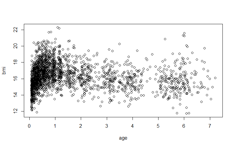
with(dat, plot(age, bmi))

dat %>% group_by(sex) %>% summarise(N = n_distinct(id))

## # A tibble: 2 × 2
##   sex       N
##   <fct> <int>
## 1 F       100
## 2 M       100

dat %>%
  group_by(id) %>%
  count() %>%
  ungroup() %>%
  summarise(median(n), min(n), max(n))

## # A tibble: 1 × 3
##   `median(n)` `min(n)` `max(n)`
##         <dbl>    <int>    <int>
## 1          11        1       21

summary(dat$age)

##    Min. 1st Qu.  Median    Mean 3rd Qu.    Max. 
## 0.07631 0.35075 0.79967 1.61011 2.24256 7.20808

The scatter plot shows all observed BMI measurements plotted against age. The dataset contains 100 females and 100 males, each with a median of 11 repeated measurements (range: 1–21). Age ranges from roughly 1 month to about 7 years.

Create Birth Weight Groups

This dataset does not record birth weight, so we simulate one for illustration. We draw a single birth weight per child from a normal distribution (mean 3,500 g, SD 500 g) and split it into quartile groups, from Q1 (lowest) to Q4 (highest), with Q1 as the reference category.

set.seed(2024)

bwt_sim <- dat %>%
  distinct(id) %>%
  mutate(BWT = rnorm(n(), mean = 3500, sd = 500))

bwt_breaks <- quantile(bwt_sim$BWT, probs = seq(0, 1, 0.25))

dat <- dat %>%
  left_join(bwt_sim, by = "id") %>%
  mutate(BWT_q = cut(
    BWT,
    breaks = bwt_breaks,
    labels = c("Q1", "Q2", "Q3", "Q4"),
    include.lowest = TRUE
  ))

dat %>% group_by(BWT_q) %>% summarise(N = n_distinct(id)) %>% mutate(`(%)` = prop.table(N)*100)

## # A tibble: 4 × 3
##   BWT_q     N `(%)`
##   <fct> <int> <dbl>
## 1 Q1       50    25
## 2 Q2       50    25
## 3 Q3       50    25
## 4 Q4       50    25

set.seed() makes the simulation reproducible. We generate one birth weight per child (distinct(id)), cut it at its quartiles, and join the resulting group back onto every row of the long-format data. Because the simulated birth weight is unrelated to BMI by construction, this analysis is intended to demonstrate the modelling workflow for a categorical grouping variable rather than to reveal a real birth-weight effect — we would expect the four groups to follow essentially the same trajectory.

1 – Natural Spline LME: Sex Differences in BMI Trajectory

To formally test whether BMI trajectories differ between sexes, we fit a combined model with an interaction between the natural spline of age and sex. This allows the entire shape of the trajectory to differ between females and males. We try 3 to 6 degrees of freedom and select the best-fitting model by BIC.

ns_mf <- map(3:6, possibly(~ {
  eval(parse(text = paste0(
    "lmer(bmi ~ ns(age, ", .x, ") * sex + (age | id),
    REML = FALSE, data = dat)"
  )))
}, otherwise = NA_real_))

df_best <- (3:6)[which.min(unlist(map(ns_mf, BIC)))]
(ns_mf_best <- ns_mf[[which.min(unlist(map(ns_mf, BIC)))]])

## Linear mixed model fit by maximum likelihood  ['lmerModLmerTest']
## Formula: bmi ~ ns(age, 5) * sex + (age | id)
##    Data: dat
##       AIC       BIC    logLik -2*log(L)  df.resid 
##  5261.728  5352.078 -2614.864  5229.728      2078 
## Random effects:
##  Groups   Name        Std.Dev. Corr  
##  id       (Intercept) 1.2348         
##           age         0.2846   -0.33 
##  Residual             0.6632         
## Number of obs: 2094, groups:  id, 200
## Fixed Effects:
##      (Intercept)       ns(age, 5)1       ns(age, 5)2       ns(age, 5)3  
##         14.59730           2.81813           2.08979           0.05257  
##      ns(age, 5)4       ns(age, 5)5              sexM  ns(age, 5)1:sexM  
##          2.98414           1.03194           0.48497          -0.45665  
## ns(age, 5)2:sexM  ns(age, 5)3:sexM  ns(age, 5)4:sexM  ns(age, 5)5:sexM  
##         -0.32209          -0.66083          -0.65169          -1.22333

What this code does:

ns(age, df) creates a natural cubic spline basis for age with df degrees of freedom. Each additional df adds one internal knot, allowing the curve to change direction one more time.
ns(age, df) * sex expands to ns(age, df) + sex + ns(age, df):sex. The interaction terms allow each spline basis coefficient to differ by sex, meaning the entire shape of the BMI trajectory can differ between females and males — not just a constant vertical offset.
(age | id) specifies a random intercept and a random slope for age within each child, allowing each child’s trajectory to deviate from the population mean in both starting level and rate of change.
REML = FALSE fits by maximum likelihood, required so that models with different fixed effects can be fairly compared using information criteria.
map(3:6, ...) fits one model for each df value from 3 to 6. possibly() returns NA for any model that fails to converge rather than stopping execution, and which.min(... BIC) selects the model with the lowest Bayesian Information Criterion (BIC). df_best stores the selected df so the same spline complexity can be reused in Section 2.

Reading the random effects output:

id (Intercept) SD: between-person variation in predicted BMI at age zero (approximately birth), i.e. how much children differ in their starting BMI level.
id age SD: between-person variation in the rate of BMI change over time.
Corr: the correlation between a child’s baseline BMI level and their rate of change.
Residual SD: within-person variation not explained by the model.

Reading the fixed effects output: The individual spline basis coefficients (e.g. ns(age, df)1) are not directly interpretable as slopes — they represent the weights of each basis function and only have meaning in combination. The corresponding ns(age, df)k:sexM interaction coefficients are likewise not individually interpretable. The shape of each sex’s trajectory, and the difference between them, is best understood through the predicted and difference plots below.

Interpretation: BIC selected 5 degrees of freedom (4 internal knots) as the best fitting model. The basis coefficients (ns(age, 5)1–5) and their :sexM counterparts should not be read as slopes or as a sex contrast on their own; they only describe the curve in combination, which is why we turn to the plots. The random effects read as in the linear spline model: children’s predicted BMI at age zero is spread with an SD of about 1.23 kg/m², their rate of change with an SD of 0.28 kg/m²/year, the two vary together with a mild negative correlation (−0.33, a description rather than a mechanism), and about 0.66 kg/m² of within-child variation remains around each personal curve.

Knot Positions

attr(terms(ns_mf_best), "predvars")

## list(bmi, ns(age, knots = c(0.2833373708, 0.5807503106, 1.126253912, 
## 3.0883893664), Boundary.knots = c(0.07630629, 7.208082142), intercept = FALSE), 
##     sex)

By default, ns() places internal knots at equally spaced quantiles of the observed age distribution. The boundary knots are fixed at the minimum and maximum observed ages.

P-value for Sex Interaction Term

anova(ns_mf_best)[3, ]

## Type III Analysis of Variance Table with Satterthwaite's method
##                Sum Sq Mean Sq NumDF  DenDF F value    Pr(>F)    
## ns(age, 5):sex 15.023  3.0046     5 806.65  6.8322 2.968e-06 ***
## ---
## Signif. codes:  0 '***' 0.001 '**' 0.01 '*' 0.05 '.' 0.1 ' ' 1

The F-test for the ns(age, ...):sex interaction (row 3 of the anova() table, with Satterthwaite degrees of freedom from lmerTest) is an omnibus test of whether the shape of the BMI trajectory differs between females and males beyond a constant vertical offset.

Interpretation: With F(5, 806.65) = 6.83 and p ≈ 0.000003, the data are not very compatible with the two sexes sharing one curve shape: how BMI changes with age appears to differ between females and males beyond a simple up-or-down shift. Because it is an omnibus test, it pools all five basis-by-sex terms and does not say at which ages the curves differ — for that, read the predicted and difference plots that follow.

Predicted Mean BMI Trajectory by Sex

predict_response(ns_mf_best,
                 terms  = c("age [all]", "sex [all]"),
                 margin = "marginalmeans") %>%
  plot() +
  ggtitle("Predicted Mean BMI Natural Spline Trajectory by Sex") +
  theme_classic()

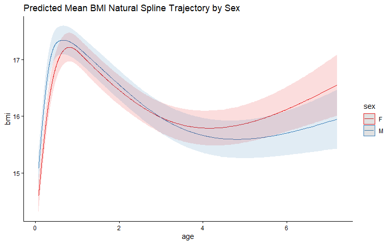
Plotting both sexes on the same axes allows direct visual comparison of the trajectories. The shaded bands are 95% confidence intervals for each sex-specific mean.

Interpretation: Read the two smooth curves as the average trajectory for each sex. Both rise to an infant peak near 0.7–0.9 years and fall to a low point around ages 4–5, but the sexes are ordered differently at different ages: males sit slightly higher through infancy and into the toddler years, the curves cross at around age 3–4, and females sit higher with a stronger upturn by age 7. This change in ordering across age — rather than one curve sitting uniformly above the other — is what the spline-by-sex interaction captures. The bands overlap through mid-childhood and widen at the youngest and oldest ages, so the separation is read most confidently where the curves are both far apart and tightly estimated.

Mean Difference in Predicted BMI (Males minus Females) by Age

Because the natural spline basis coefficients are not directly interpretable, we use comparisons() to estimate the sex difference in predicted mean BMI at each age directly, with confidence intervals.

pred_diff <- comparisons(
  ns_mf_best,
  variables = "sex",
  newdata   = datagrid(age = seq(0.5, 7, by = 0.5))
) %>% as.data.frame()

ggplot(data = pred_diff,
       aes(x = age, y = estimate, ymin = conf.low, ymax = conf.high)) +
  theme_classic() +
  geom_pointrange(size = 0.25) +
  geom_hline(yintercept = 0, lty = 2, col = "red", linewidth = 0.1) +
  scale_x_continuous(breaks = seq(0, 7, by = 1)) +
  xlab("Age (years)") +
  ylab("Predicted mean difference (Males minus Females)")

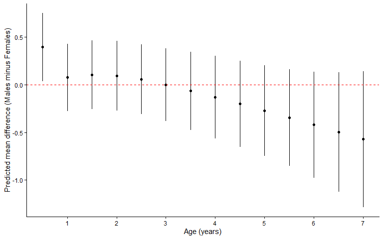
Reading the plot:

Each point is the estimated difference in predicted mean BMI (males minus females) at that age, with a 95% confidence interval.
The red dashed line at zero is the reference for no sex difference.
Points above the line indicate higher BMI in males; points below indicate higher BMI in females.
Ages where the confidence interval does not cross the red line indicate a statistically meaningful sex difference at that age.

Interpretation: This plot localises the sex contrast that the omnibus test flagged. The males-minus-females difference starts slightly positive in early infancy (about +0.4 kg/m² at 6 months, the one age whose interval sits just clear of zero), stays close to zero through the toddler and preschool years, and drifts negative (females higher) toward age 7. So the point estimates trace a gradual crossover with age, but every interval except the earliest includes zero, and they widen markedly at the oldest ages where data are sparse. The two readings sit together comfortably: the shape of the trajectory differs by sex (omnibus test), yet the age-specific gaps are estimated too imprecisely to pin down at most individual ages.

2 – Natural Spline LME: Effect of Birth Weight on BMI Trajectory

We extend the model to include an interaction between the natural spline of age and the (simulated) birth weight quartile group (BWT_q). This allows the shape of the BMI trajectory to differ across the four birth weight groups, while still adjusting for sex. We reuse the spline complexity (df_best) selected by BIC in Section 1, so that both models use the same basis.

(ns_mf_bw <- eval(parse(text = paste0(
  "lmer(bmi ~ ns(age, ", df_best, ") * (sex + BWT_q) + (age | id),
   REML = FALSE, data = dat)"
))))

## Linear mixed model fit by maximum likelihood  ['lmerModLmerTest']
## Formula: bmi ~ ns(age, 5) * (sex + BWT_q) + (age | id)
##    Data: dat
##       AIC       BIC    logLik -2*log(L)  df.resid 
##  5272.821  5464.813 -2602.411  5204.821      2060 
## Random effects:
##  Groups   Name        Std.Dev. Corr  
##  id       (Intercept) 1.2319         
##           age         0.2834   -0.33 
##  Residual             0.6589         
## Number of obs: 2094, groups:  id, 200
## Fixed Effects:
##         (Intercept)          ns(age, 5)1          ns(age, 5)2  
##            14.69746              2.48466              2.05164  
##         ns(age, 5)3          ns(age, 5)4          ns(age, 5)5  
##            -0.07335              2.59796              0.68276  
##                sexM              BWT_qQ2              BWT_qQ3  
##             0.51925             -0.19023              0.10091  
##             BWT_qQ4     ns(age, 5)1:sexM     ns(age, 5)2:sexM  
##            -0.37750             -0.48137             -0.35027  
##    ns(age, 5)3:sexM     ns(age, 5)4:sexM     ns(age, 5)5:sexM  
##            -0.66928             -0.68207             -1.21862  
## ns(age, 5)1:BWT_qQ2  ns(age, 5)2:BWT_qQ2  ns(age, 5)3:BWT_qQ2  
##             0.66088              0.22748              0.08605  
## ns(age, 5)4:BWT_qQ2  ns(age, 5)5:BWT_qQ2  ns(age, 5)1:BWT_qQ3  
##             0.47893              0.51900              0.29402  
## ns(age, 5)2:BWT_qQ3  ns(age, 5)3:BWT_qQ3  ns(age, 5)4:BWT_qQ3  
##            -0.26146              0.26705              0.30820  
## ns(age, 5)5:BWT_qQ3  ns(age, 5)1:BWT_qQ4  ns(age, 5)2:BWT_qQ4  
##             0.41462              0.41138              0.24618  
## ns(age, 5)3:BWT_qQ4  ns(age, 5)4:BWT_qQ4  ns(age, 5)5:BWT_qQ4  
##             0.15114              0.84601              0.48788

Writing the spline once and interacting it with (sex + BWT_q) is equivalent to interacting it with each separately, but keeps a single ns(age, ...) basis in the model — this avoids a duplicated spline term that can confuse the marginal-means machinery used for the plot below. The specification adds main effects for groups Q2, Q3 and Q4 (each relative to the Q1 reference group) plus a set of basis-by-group interaction terms. As with the sex interaction, the individual ns(age, ...)k:BWT_qQ# coefficients are not directly interpretable in isolation; their combined effect on each group’s trajectory is best read from the predicted plot below.

P-value for Birth Weight Interaction Term

anova(ns_mf_bw)[5, ]

## Type III Analysis of Variance Table with Satterthwaite's method
##                  Sum Sq Mean Sq NumDF  DenDF F value  Pr(>F)  
## ns(age, 5):BWT_q 10.375 0.69165    15 810.42  1.5933 0.06959 .
## ---
## Signif. codes:  0 '***' 0.001 '**' 0.01 '*' 0.05 '.' 0.1 ' ' 1

The F-test for ns(age, ...):BWT_q (row 5 of the anova() table) is an omnibus test of whether birth weight modifies the shape of the BMI trajectory — i.e. whether the trajectory shape differs significantly across the four birth weight groups. A significant result indicates that the association between birth weight and BMI is not constant across childhood but varies in magnitude or direction at different ages.

Interpretation: The joint test of all 15 basis-by-group terms gives F(15, 810.42) = 1.59, p ≈ 0.07.

Predicted Mean BMI Trajectory by Birth Weight Quartile

predict_response(ns_mf_bw,
                 terms  = c("age [0.08:7.2 by=0.1]", "BWT_q"),
                 margin = "marginalmeans") %>%
  plot() +
  ggtitle("Predicted Mean BMI Natural Spline Trajectory by Birth Weight Quartile") +
  theme_classic()

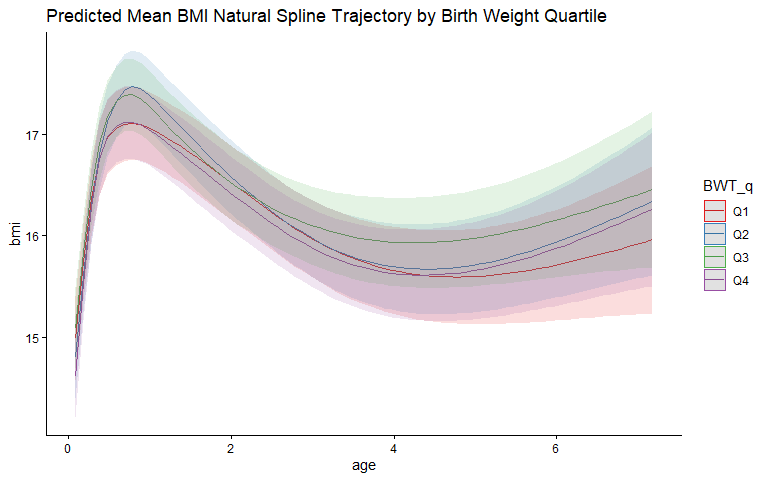
Each line is the predicted mean BMI trajectory for one birth weight group, from Q1 (lowest) to Q4 (highest), with shaded 95% confidence bands. Periods where the curves run parallel indicate no birth-weight-by-age interaction at that age; periods where they converge, diverge, or cross indicate that the association between birth weight and BMI changes with age.

Interpretation: The four quartile curves overlap throughout and there is no indication that the BMI trajectory differs by birth weight quartile.

Summary

In this tutorial we fitted natural cubic spline LME models to characterise the mean BMI trajectory from infancy to early school age. Key points:

Natural splines provide a flexible, well-behaved alternative to polynomials for modelling nonlinear trajectories, constrained to be linear beyond the boundary knots.
The number of degrees of freedom (and therefore knot positions) was selected by BIC, balancing model fit against complexity, and the selected complexity was reused across both analyses.
A combined model with a sex-by-spline interaction allowed formal estimation of the sex difference in predicted BMI at each age, with confidence intervals, since the individual spline coefficients are not directly interpretable.
Extending the model to include a birth-weight-group-by-spline interaction (simulated groups Q1–Q4, entered as a categorical factor) demonstrated how group differences in trajectory shape would be tested, while adjusting for sex.

On this page